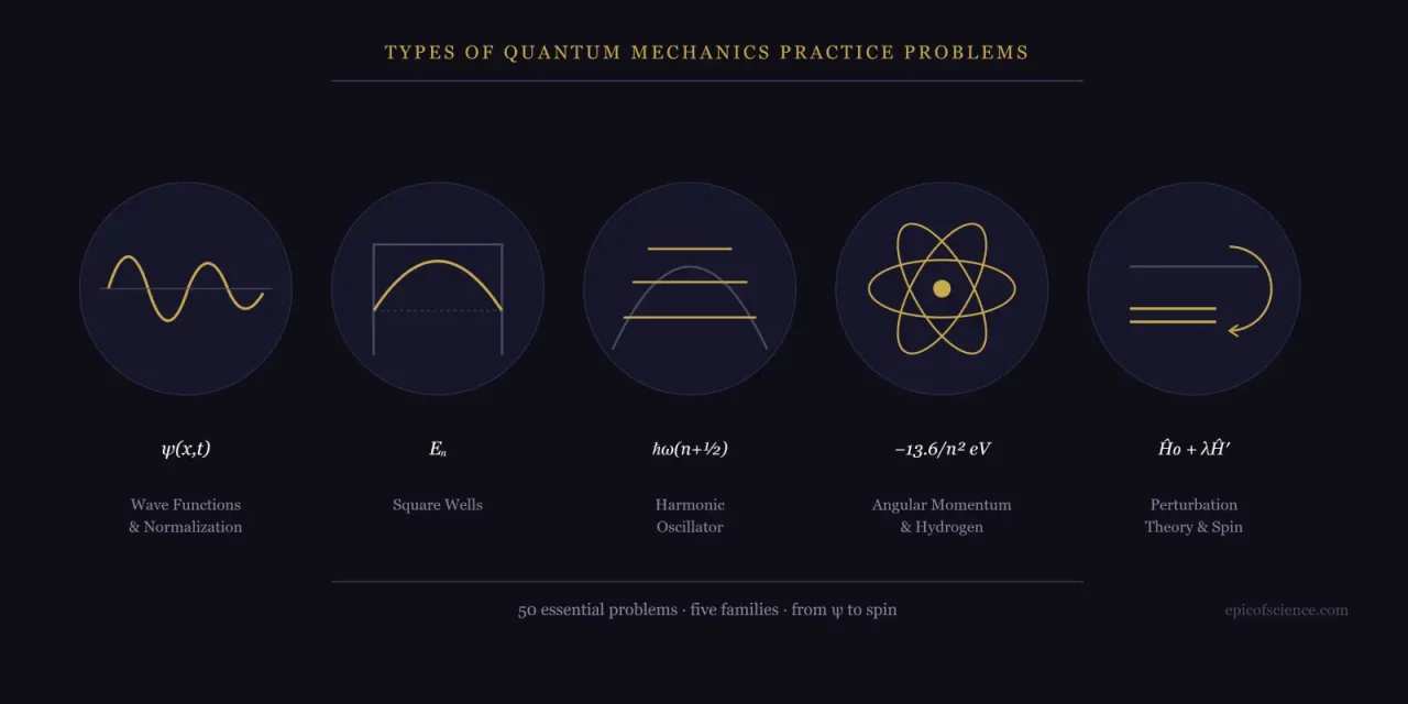
These quantum mechanics practice problems are arranged so that by the last one you can normalize a wave function and read a probability directly, solve the infinite square well and evolve a superposition through time, handle the harmonic oscillator entirely with ladder operators, extract the hydrogen spectrum and angular momentum from a single energy level, and compute a first-order energy shift alongside a spin measurement. Each type is presented the same way: a concrete problem with real functions and numbers, a full solution worked line by line, and the trap that most often costs students marks.
The five sections move from the lightest algebra to the most involved machinery. Within each one, the reasoning is spelled out rather than compressed. You are not meant to skim. The value of quantum mechanics practice problems comes from doing, so treat each worked solution as an answer key you consult only after your own honest attempt. Formalism is presented as formalism throughout: where the Schrödinger equation or the Born rule enters, it is named for what it is, without any interpretive gloss dressed up as mathematical fact.
How to Use This Guide
Keep three things within arm’s reach before you begin. The first is the time-independent Schrödinger equation \( \hat{H}\psi = E\psi \), which fixes the stationary states and their energies for every bound system below. The second is the Born rule: the modulus squared of a normalized wave function is a probability density, so \( \int |\psi|^2\,dx = 1 \). This rule is an axiom of the theory, not a derived result or tied to any single interpretation of what the wave function “is.” The third is enough calculus to integrate exponentials, Gaussians, and products of sines, which is most of what these calculations demand.
Quantum mechanics practice problems are structured exercises that ask you to apply the Schrödinger equation, normalization, and operator algebra to concrete physical systems — wells, oscillators, atoms, spins — and produce a definite result, such as an energy, a probability, or an expectation value, testing both your computation and your physical understanding.
Two smaller habits pay off across every problem below. The first is to check dimensions at the end: energy must come out in energy units, probability must be a pure number between zero and one, and length must be a length. A quick dimensional glance catches most dropped factors before they harden into a wrong answer. The second is to test limiting cases whenever a symbol is left general, asking what the result becomes as a width grows large, a mass grows heavy, or a quantum number climbs, and comparing that limit against physical intuition.
The single habit that separates learning from watching is attempting the problem first. Read the statement, close the solution, and push as far as you can on paper before checking a single line. When stuck, uncover one step, then cover it again and continue on your own. Worked quantum physics practice problems teach method only when your own attempt has exposed where the method was needed, so resist reading passively and let each solution confirm or correct a decision you have already made.
Wave Functions and Normalization
This is where every quantum calculation starts, so practice should start here too. Before asking a particle’s momentum or position, the state must be normalized because the Born rule assigns probabilities only to wave functions whose modulus squared integrates to one. Wave function problems reward a small, reliable ritual: write the normalization condition, substitute, integrate, solve for the constant, and then compute whatever the question asks.
A particle moves in one dimension with the unnormalized wave function \( \psi(x) = A\,e^{-|x|/a} \), where \( a \gt 0 \) is a fixed length. Find the constant \( A \) that normalizes \( \psi \), then compute the probability of finding the particle within one decay length of the origin, that is, in the region \( |x| \lt a \).
Begin with the normalization condition, which is the Born rule written as a demand on the whole line.
\[ \int_{-\infty}^{\infty} |\psi(x)|^2\,dx = 1 \]
Substitute the wave function. Because the integrand \( e^{-2|x|/a} \) is even, the integral over the whole line equals twice the integral over the positive half, removing the absolute value.
\[ |A|^2 \int_{-\infty}^{\infty} e^{-2|x|/a}\,dx = |A|^2 \cdot 2\int_{0}^{\infty} e^{-2x/a}\,dx \]
The remaining integral is a standard decaying exponential, and it evaluates cleanly.
\[ 2\int_{0}^{\infty} e^{-2x/a}\,dx = 2\left[-\tfrac{a}{2}\,e^{-2x/a}\right]_{0}^{\infty} = a \]
Setting the whole thing equal to 1 gives the normalization constant, taken as real and positive by convention.
\[ |A|^2 a = 1 \quad\Longrightarrow\quad A = \frac{1}{\sqrt{a}} \]
Now the physical question. The probability of finding the particle within one decay length is the integral of the probability density over \( -a \lt x \lt a \), and by the same even-function argument, it doubles the half-range integral.
\[ P(|x|\lt a) = \frac{1}{a}\int_{-a}^{a} e^{-2|x|/a}\,dx = \frac{2}{a}\int_{0}^{a} e^{-2x/a}\,dx = 1 – e^{-2} \approx 0.865 \]
So about eighty-six percent of the probability lives within a single decay length of the origin, which matches the physical picture of a state sharply peaked at \( x=0 \). The trap here is integrating \( \psi \) itself rather than \( |\psi|^2 \); probability comes from the modulus squared, never from the amplitude. The second trap is forgetting the factor of two that the absolute value hides, which quietly halves your answer and makes the state look unnormalizable.
The Infinite and Finite Square Well
The square well is the workhorse of Schrödinger equation practice because its stationary states are just sines and its energies are pure algebra. The infinite well confines the particle absolutely, quantizing the energy through the boundary conditions at the walls; the finite well relaxes those walls, so the wave function leaks into the classically forbidden region, and the allowed energies come from a transcendental matching condition rather than a tidy formula. In the finite case, you match the wave function and its derivative at each wall, and the resulting equation has only a handful of solutions, so a shallow or narrow well may hold just one or two bound states rather than the infinite ladder of the ideal well. The worked problem below uses the infinite well, whose exact states make it the right place to practice superposition and time evolution before the finite-well algebra is layered on top.
A particle of mass \( m \) sits in an infinite square well of width \( L \), with walls at \( x=0 \) and \( x=L \). At \( t=0 \) it is prepared in the state \( \Psi(x,0) = A\big[\psi_1(x) + \psi_2(x)\big] \), where \( \psi_n \) are the normalized stationary states. Find \( A \), write the state \( \Psi(x,t) \) at later times, and compute the expectation value of the energy.
Recall the stationary states and their energies, which solve the time-independent Schrödinger equation inside the well and vanish at both walls.
\[ \psi_n(x) = \sqrt{\frac{2}{L}}\,\sin\!\left(\frac{n\pi x}{L}\right), \qquad E_n = \frac{n^2\pi^2\hbar^2}{2mL^2} \]
Normalize the superposition. Because the stationary states are orthonormal, the cross terms integrate to zero, and only the two unit-norm terms survive.
\[ |A|^2\big(\langle\psi_1|\psi_1\rangle + \langle\psi_2|\psi_2\rangle\big) = 2|A|^2 = 1 \quad\Longrightarrow\quad A = \frac{1}{\sqrt{2}} \]
Time evolution is obtained by attaching to each stationary state its own phase factor \( e^{-iE_n t/\hbar} \). This is the whole content of solving the time-dependent Schrödinger equation once the state is expanded in energy eigenstates.
\[ \Psi(x,t) = \frac{1}{\sqrt{2}}\Big[\psi_1(x)\,e^{-iE_1 t/\hbar} + \psi_2(x)\,e^{-iE_2 t/\hbar}\Big] \]
The expected energy is the sum of the eigenvalues weighted by the probabilities \( |c_n|^2 \), each of which is one-half here.
\[ \langle E\rangle = |c_1|^2 E_1 + |c_2|^2 E_2 = \tfrac{1}{2}E_1 + \tfrac{1}{2}E_2 \]
Since \( E_2 = 4E_1 \), the result follows immediately.
\[ \langle E\rangle = \tfrac{1}{2}\big(E_1 + 4E_1\big) = \frac{5}{2}E_1 = \frac{5\pi^2\hbar^2}{4mL^2} \]
Notice that \( \langle E\rangle \) is not an energy the particle can ever be measured to have; a measurement yields \( E_1 \) or \( E_2 \), each with probability one half, and the expectation value is only their average. The most common mistake in these quantum mechanics exercises is expecting the time-dependent phases to change something measurable about energy — they do not, because \( |c_n|^2 \) is untouched by a pure phase, so the energy statistics are frozen for this closed system even as the probability density visibly sloshes.
The Harmonic Oscillator and Ladder Operators
The harmonic oscillator is worth mastering algebraically rather than through brute integration, because the ladder operators turn every expectation value into bookkeeping about how \( a_+ \) and \( a_- \) raise and lower states. Once you internalize their action, you never touch a Hermite polynomial again. The following problem is the canonical check that the ground state sits exactly at the floor set by the uncertainty principle, and it is among the most instructive quantum mechanics exercises for building operator fluency.
For the harmonic oscillator with Hamiltonian \( \hat{H} = \dfrac{\hat{p}^2}{2m} + \tfrac{1}{2}m\omega^2 \hat{x}^2 \), work entirely in terms of the ladder operators to compute \( \Delta x \) and \( \Delta p \) in the ground state \( |0\rangle \), and verify that their product saturates the uncertainty relation.
Write position and momentum in terms of the ladder operators. Carry the factor of \( i \) in the momentum carefully; dropping it is the fastest way to a negative variance.
\[ \hat{x} = \sqrt{\frac{\hbar}{2m\omega}}\,(a_+ + a_-), \qquad \hat{p} = i\sqrt{\frac{m\omega\hbar}{2}}\,(a_+ – a_-) \]
The operators act as \( a_-|0\rangle = 0 \), \( a_+|n\rangle = \sqrt{n+1}\,|n+1\rangle \), and \( a_-|n\rangle = \sqrt{n}\,|n-1\rangle \), with the commutator \( [a_-, a_+] = 1 \). By the symmetry of the ground state, \( \langle x\rangle = \langle p\rangle = 0 \), so each variance is just the expectation of the square.
\[ \langle x^2\rangle = \frac{\hbar}{2m\omega}\,\langle 0|(a_+ + a_-)^2|0\rangle \]
Expand the square into \( a_+^2 + a_+a_- + a_-a_+ + a_-^2 \). Acting on \( |0\rangle \), the terms ending in \( a_- \) vanish, and \( a_+^2|0\rangle \) is proportional to \( |2\rangle \), which is orthogonal to \( |0\rangle \). Only \( a_-a_+ \) survives.
\[ \langle 0|(a_+ + a_-)^2|0\rangle = \langle 0|a_-a_+|0\rangle = 1 \quad\Longrightarrow\quad \langle x^2\rangle = \frac{\hbar}{2m\omega} \]
The momentum follows the same pattern, with the sign from \( i^2 = -1 \) turning the surviving term positive.
\[ \langle p^2\rangle = -\frac{m\omega\hbar}{2}\,\langle 0|(a_+ – a_-)^2|0\rangle = \frac{m\omega\hbar}{2} \]
The product of the standard deviations is then exactly the Heisenberg floor.
\[ \Delta x\,\Delta p = \sqrt{\frac{\hbar}{2m\omega}}\;\sqrt{\frac{m\omega\hbar}{2}} = \frac{\hbar}{2} \]
The ground state is the minimum-uncertainty state, saturating \( \Delta x\,\Delta p \ge \hbar/2 \) with equality. That is not a coincidence tuned by hand; it is why the oscillator has a zero-point energy at all, since a state pinned to the bottom of the well would violate the very inequality the ground state only just meets. The trap here is treating \( a_+ \) and \( a_- \) as if they commute; because \( a_-a_+ \) and \( a_+a_- \) differ by one, the order inside the square is what selects the surviving term. Get the ordering wrong and the variance collapses to zero or turns negative, which should always read as a signal that a commutator was mishandled rather than a real result.
Angular Momentum and the Hydrogen Atom
Hydrogen is where quantization stops being abstract and starts predicting colors you can see. The orbital angular momentum sets the shape of each state through the quantum numbers \( \ell \) and \( m \), while the energy depends only on \( n \), and the difference between two energy levels is a photon with a definite wavelength. Practicing here means holding two quantizations at once — of angular momentum and of energy — inside a single level, which is exactly what the problem below asks. These quantum physics problems and solutions are the ones that connect equations to spectroscopy.
Consider the \( n=3 \) level of hydrogen. First, for an electron in the \( \ell = 2 \) state, find the magnitude of the orbital angular momentum, its allowed \( z \)-components, and the smallest angle \( \vec{L} \) can make with the \( z \)-axis. Then find the wavelength of the photon emitted in the \( n=3 \to n=2 \) transition.
The magnitude of orbital angular momentum is fixed by \( \ell \), and the crucial point is that it depends on \( \ell(\ell+1) \), not on \( \ell \) alone.
\[ |\vec{L}| = \hbar\sqrt{\ell(\ell+1)} = \hbar\sqrt{2\cdot 3} = \sqrt{6}\,\hbar \]
The \( z \)-component is quantized in integer steps of \( \hbar \) from \( -\ell \) to \( +\ell \).
\[ L_z = m\hbar, \qquad m = -2,\,-1,\,0,\,1,\,2 \]
The angle with the axis is smallest when \( L_z \) is largest, so set \( m = 2 \) and take the ratio.
\[ \cos\theta_{\min} = \frac{L_z^{\max}}{|\vec{L}|} = \frac{2\hbar}{\sqrt{6}\,\hbar} = \frac{2}{\sqrt{6}} \quad\Longrightarrow\quad \theta_{\min} \approx 35.3^\circ \]
Because \( \sqrt{6} \gt 2 \), the vector can never point fully along the axis; there is always a residual tilt, a direct fingerprint of the uncertainty in the transverse components. Now the transition. Hydrogen’s bound-state energies carry a negative sign, the mark of a bound electron.
\[ E_n = -\frac{13.6\ \text{eV}}{n^2} \]
The emitted photon carries the energy difference between the initial and final levels.
\[ E_\gamma = E_3 – E_2 = -13.6\left(\frac{1}{9} – \frac{1}{4}\right)\text{eV} = 13.6\cdot\frac{5}{36}\ \text{eV} \approx 1.89\ \text{eV} \]
Convert energy to wavelength with \( hc \approx 1240\ \text{eV·nm} \).
\[ \lambda = \frac{hc}{E_\gamma} = \frac{1240\ \text{eV·nm}}{1.89\ \text{eV}} \approx 656\ \text{nm} \]
That is the red H-alpha line of the Balmer series, a result you can verify against any spectral chart.

Image: Wikimedia Commons, CC0 (public domain).
The four visible Balmer lines. The red one at 656 nm is the photon worked out above — the n = 3 to n = 2 transition, measured rather than assumed.
The trap that ruins this problem is writing \( |\vec{L}| = \ell\hbar \) instead of \( \sqrt{\ell(\ell+1)}\,\hbar \); the two agree for large \( \ell \) but differ sharply for the small values that matter. The second trap is mishandling the negative sign in the energies and reporting a negative photon energy — the photon carries away the positive difference.
Perturbation Theory and Spin
Perturbation theory is how you make progress when the Hamiltonian is almost, but not quite, one you can solve, and its first-order result is disarmingly simple: the energy shift is the expectation value of the perturbation in the unperturbed state. Spin, meanwhile, is the cleanest arena for the measurement postulate, because the state lives in two dimensions and every probability is a squared component. Pairing them makes for compact quantum mechanics solved problems that drill both the correction formula and the Born rule at once.
Return to the infinite square well of width \( L \), now with a narrow spike at its center modeled by \( H’ = \alpha\,\delta(x – L/2) \). Find the first-order correction to every energy level. Then, separately, a spin-\( \tfrac{1}{2} \) particle is in the state \( \chi = \frac{1}{\sqrt{5}}\begin{pmatrix}1\\2\end{pmatrix} \) written in the \( S_z \) basis; find the probability of measuring \( S_z = +\hbar/2 \) and the expectation value \( \langle S_z\rangle \).
The first-order shift is the expectation value of \( H’ \) in the unperturbed state, and the delta function simply evaluates the density at the center of the well.
\[ E_n^{(1)} = \langle\psi_n|H’|\psi_n\rangle = \alpha\,|\psi_n(L/2)|^2 = \alpha\cdot\frac{2}{L}\sin^2\!\left(\frac{n\pi}{2}\right) \]
The sine at the midpoint is \( \pm 1 \) for odd \( n \) and exactly zero for even \( n \), which splits the answer into two clean cases.
\[ E_n^{(1)} = \begin{cases} \dfrac{2\alpha}{L}, & n \ \text{odd} \\[2mm] 0, & n \ \text{even} \end{cases} \]
The even states are untouched because each has a node precisely at the center, where the spike sits, so they never feel it — a result you could have guessed from the geometry before doing any algebra. Turning to spin, the state is already normalized since \( (1 + 4)/5 = 1 \), so the probability of the spin-up outcome is the squared modulus of the upper component.
\[ P\!\left(S_z = +\tfrac{\hbar}{2}\right) = \left|\frac{1}{\sqrt{5}}\right|^2 = \frac{1}{5}, \qquad P\!\left(S_z = -\tfrac{\hbar}{2}\right) = \frac{4}{5} \]
The expectation value is the average of the two eigenvalues weighted by those probabilities.
\[ \langle S_z\rangle = \frac{1}{5}\cdot\frac{\hbar}{2} + \frac{4}{5}\cdot\left(-\frac{\hbar}{2}\right) = -\frac{3\hbar}{10} \]
Two traps lurk here. In perturbation theory, the simple first-order formula holds only when the level is non-degenerate; a degenerate level requires you to first diagonalize \( H’ \) within the degenerate subspace, or the answer is meaningless. In the spin measurement, the amplitude \( 1/\sqrt{5} \) is not the probability — you must square it — and the state must be normalized before any component is squared, or the probabilities will not sum to one.
Where to Go Next
The fastest way to consolidate these five types is to rework each problem with the numbers changed — a different well width, a heavier particle, a spin state with a complex component — until the method survives without the specific values propping it up. From there, widen the net. After normalization and expectation values, practice time evolution of genuine wave packets and the Ehrenfest relations that connect them to classical motion. After the infinite well, solve the finite well’s transcendental condition numerically and count its bound states. After the ladder operators, use them for the coherent states that remain in minimal uncertainty as they oscillate. After hydrogen, add the spin-orbit and relativistic corrections that produce fine structure, which is where perturbation theory earns its keep.
Working a steady diet of quantum physics practice problems across these directions is what turns isolated tricks into a single flexible method. For a deeper library of quantum physics problems and solutions grouped by exactly these themes, the problem sets and solutions from MIT OpenCourseWare 8.04 are an authoritative, freely available source to test yourself against. To keep building the surrounding physics that makes these calculations meaningful, continue with more explainers and worked material in the physics section of Epic of Science, where the concepts behind these quantum mechanics exercises are developed in fuller narrative form.
Keep Practicing
The method never changes, only the system it is aimed at. Attempt the problem cold, push the algebra as far as it will go, and only then check your work against the worked solution — not to see whether you got the number, but to see whether your reasoning matched the reasoning, step for step. When they diverge, that gap is the actual lesson, and it is worth more than any answer. Return to these quantum mechanics practice problems whenever a new topic feels slippery; normalization, the wells, the oscillator, hydrogen, and perturbation with spin are the load-bearing skills that everything harder is built on. Understand the why behind each step, and the next set of problems, however unfamiliar it looks at first, will yield to the same patient approach.
MIT OpenCourseWare, 8.04 Quantum Physics I (Spring 2016), Assignments and Solutions.
- J. Griffiths and D. F. Schroeter, Introduction to Quantum Mechanics, 3rd ed.
- Zettili, Quantum Mechanics: Concepts and Applications, 2nd ed.




Trackbacks/Pingbacks